Determining uncertainty, part 2
How to teach an AI to question itself

(You haven't read part 1 yet? Find the first article here: "Uncertainties we can rely on")

For the processes being tested here, the focus is on image classification in order to keep the number of potential factors that could influence the analyses to a minimum. The job of the DNNs is to determine the correct category, e.g. pedestrian or car, for various different images.

Sampling-based processes

The first and probably best known method of determining uncertainty for DNNs is called Monte-Carlo-Dropout. This requires the DNN to be trained using the dropout regularization method before it is used. This method deactivates individual neurons with a given probability at each step of the training. This is in contrast to the conventional approach, in which no neurons are deactivated during the prediction stage. In Monte Carlo dropout, the DNN is shown the same images multiple times, but with different neurons deactivated. This allows the results of the individual runs to be combined in order to approximate the actual probability distribution across categories. The mean and variance of this distribution can then be used as a measure of uncertainty. Conventional classification using the softmax function, on the other hand, simply uses a point estimate of probability. This cannot reliably be used to determine uncertainty — empirical analyses have shown that it returns significantly exaggerated confidence values.

Monte Carlo dropout is similar to a method known as the deep ensembles method. The core idea is to train the same DNN on the same data but with its neuron weights initialized differently so that they converge on different local minimums. Finally, to make the prediction, an ensemble is formed from the DNNs and the individual predictions are combined. As a result, this also produces a mean and variance for the different predictions of the individual DNNs.

Non-sampling-based processes

The two methods described above are sampling-based processes, requiring a single, combined prediction from multiple prediction steps to determine uncertainty. For performance reasons, these processes may be unsuitable for lower-performance embedded systems in particular. We have therefore examined another two methods that can each be executed using just one prediction step.

The first non-sampling-based process, learned confidence, learns the confidence for a prediction explicitly. As in the other methods, this is achieved by a part of the network learning the correct classifications for the input images. However, there is also a second part to the network, which is trained to predict as accurately as possible how certain the network is of its classification.

Evidential deep learning, meanwhile, brings ideas from evidence theory to DNNs. Specifically, instead of the usual classification using softmax, this method works by learning the parameters of a Dirichlet distribution and then using these for the prediction. This is intended to produce better calibrated probabilities between the categories and an overall uncertainty for the prediction.

Autonomous systems: Which process is the most convincing?

The methods presented above have different advantages and disadvantages, and have to some extent already been compared in terms of their general properties. However, there has been little research so far into the concrete added value that can be offered by the processes, for example in the context of the Fraunhofer IKS four-plus-one security architecture. Establishing this added value is the starting point for our work.

If uncertainty is incorporated into a prediction by a DNN, the evaluation includes not only the dimension “true and false” but also “certain and uncertain”. Whether a DNN is certain or uncertain is dependent on a threshold value. For example, the decisions made by a DNN may be classified as certain when the uncertainty value is below 20%, and as uncertain in all other cases. In total, there are four ways in which a decision can be evaluated:

• certain and true,
• certain and false,
• uncertain and true,
• uncertain and false

For the system as a whole, the incorporation of uncertainty means that fewer mistakes are made because predictions that are uncertain and false can be filtered out. However, predictions that are uncertain but actually true are also rejected, leading to a reduction in the overall performance of the system.

New and meaningful metrics

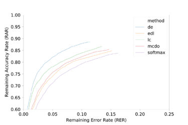
To make this trade-off easier to understand, we have defined two new metrics: the remaining error rate (RER) and the remaining accuracy rate (RAR). Both of these assume that uncertain predictions are filtered out. The RER specifies the number of remaining false predictions relative to the total number of predictions, and the RAR specifies the number of remaining true predictions relative to the total.

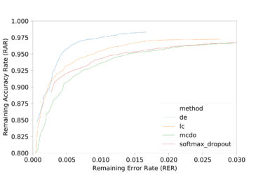
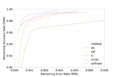
When these are calculated and visualized as a whole, using different thresholds to classify predictions as certain or uncertain, different characteristics of the individual processes become clear:

The graphs show that it is possible to reduce the error rate significantly, but that this results in very high performance losses in some cases. This could also lead to the conclusion that deep ensembles should be used if the computing power is available. Otherwise learned confidence should be used. With other datasets, however, the picture becomes less clear:

Using different architectures once again highlights differences between the processes. The same happens when the distributional shift between training and test data needs to be taken into account. It is therefore not possible to state definitively which process is best suited to a particular use case, and the specific advantages and disadvantages always need to be weighed up. That is why Fraunhofer IKS provides support for selecting the right AI methods — just contact bd@iks.fraunhofer.de.

You can find more results from the comparison of the four state-of-the-art methods in the following paper:

Uncertainties we can rely on

Find the first part of this small blog series on uncertainty determinations here: Uncertainties we can rely on